Neural Networks: How to Build a NN Model from Scratch

Companies that know how to satisfy their customers will most likely retain those customers. And companies that retain customers tend to make more sales and grow faster.
Business profitability is directly linked to customer loyalty. Winning customer loyalty, in turn, requires that you give them the greatest satisfaction attainable. But how can we read and understand this customer satisfaction easily and in time?
Enters the Neural Network (or NN model). The neural network model was developed to stimulate brain neurons/reactions/output artificially. By stimulating these neurons, these models can then predict, accurately, how a person could behave. Applied to customers, we can then begin to see and understand what is happening in their brains and whether or not they have been satisfied enough to give us their unwavering loyalty.
This is a very fascinating yet complicated subject. One which we will try to break down in bits: from what neural network models are to how to build an easy network model from scratch.
What are Neural Networks
Neural networks are a group of computer algorithm that tries to copy and use the way the human brain works to recognize any underlying relationship that could exist within a given dataset. We may also call them simulated neural networks or artificial neural networks because they usually try to artificially simulate the biological neurons signal.
An NNmodel works by using node layers. It contains an inner layer called the input layer, single or multiple middle layers called the hidden layers as well as an outer layer called the output layer. The network modelling starts off by assuming a predicted output. Next, the input layer is determined and the weights allocated. Finally, a threshold is determined. Once the result from a layer exceeds the determined threshold, the next layer is activated and the data is passed to it. This usually continues until the data gets to the output layer. This cascading of data from one layer to another can be applied to both simple and complex decisions like we will see later in this article.
Typical NN modelling usually consists of a dataset that is divided into 2: test data and training data. The test data helps us build a model while the training data helps the neural network models learn and improve its accuracy with time.
Explanation of Neural Network Basics
Before getting started with neural networks, we need to first explain what the basics are.
A Neuron Model
The basic logistic or sigmoid unit depicted below tries to show how inputs produce an output in the human brain.
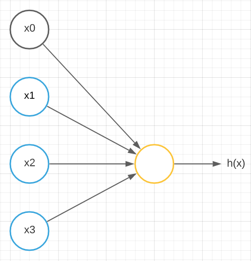
Where x0 is the bias neuron and x1, x2, and x3 are the input nodes of the input layer and h(x) is the output.
A shallow neural network typically resembles the image above but with more layers.
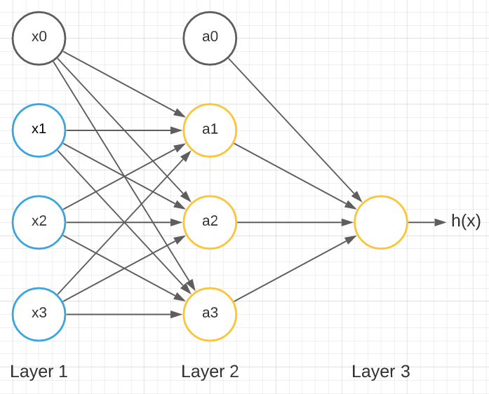
Where Layer 1 is called the input layer with x0 as the bias unit and x1, x2, and x3 as its input units. Layer 2 is called the hidden layer with a0 as the bias unit and a1, a2, and a3 as the input units for that layer. There are neural networks with more than a single hidden layer. The output layer is Layer 3.
But this is only one among the other types of neural networks. Another common type is the deep neural network which usually has more than one hidden layers.
Computation Process
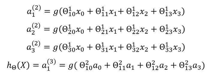
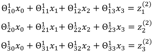
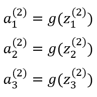
For a model to run properly, some computation steps need to happen. The first computation step is known as activation which is defined as a value resulting from a specific neuron or unit. It is described by the equations below:
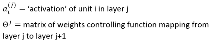
Weights
Weights are a key component of NN models. They help to determine the importance of each unit. The units assigned larger values of weight are generally considered to be more important than those with lesser values. That means if x1 in our neuron diagram above has an assigned weight of w6 and x2 has an assigned weight of w3, the x1 unit will be more influential in determining the final decision or output than x2.
The equation below describes a matrix of weights:
Each weight is multiplied by its corresponding input to give another input that fires off the activation function. The activation hits the following layer; the process is repeated until the final output of that neuron is reached.
Forward Propagation
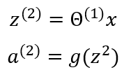
Forward propagation includes all the process we have so far described summed up; multiplying the weights and inputs and applying the activation function to reach an output. With this, we can do any modeling that suits our needs while mapping inputs and outputs to suitable weight values and their activation functions. The forward propagation can be represented by the equation below:
Back Propagation
Backpropagation moves backwards from output to input as opposed to forward propagation and is an important aspect of neural network training where we have to determine the gradient descent and then modify all the weight values to help us arrive at the desired output. The gradient descent can be determined by first knowing what the cost function is. The cost function, simply put, is the distance of the predicted output from the observed output. It shows the accuracy of an NN model so that the smaller the value of the cost function, the more accurate the model is. Once the cost function is determined, the backpropagation ensures that the weights continue to adjust until a better accuracy is achieved.
Gradient Descent
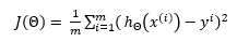
The stochastic gradient descent is generally used for increasing the accuracy of the model by determining the cost function and then multiplying it with the learning rate. The most common way of determining the cost function is by using the Mean-Squared Error depicted by the equation below:
The gradient descent can be represented by the equation shown below:
Epoch
An epoch is an instance that occurs when we have run an entire dataset through a single forward propagation and a single backward propagation.

Practical Usage of Neural Networks
There are many practical applications of a neural network but we consider just one case.
This practical usage uses the Breast Cancer dataset from the UCI’s Machine Learning Repository. All the lines of code used can be found in this GitHub repository.
First, all necessary libraries were imported into a Pandas dataframe. The dataset contained a total of 32 features and 569 data points for each feature. The features all contained information about tumors found in patients. Some of the tumors were malignant while others were benign. The work of this model was to classify which tumor was ‘Malignant’ and which was ‘Benign’ using the 32 features found.
Within the dataset, the feature known as diagnosis was determined to contain the target variable. We can use the code below to check the unique values within the target variable:
array ([‘M’, ‘B’], dtype=object)
The predicted outcomes were ‘M’ for malignant and ‘B’ for benign which can be replaced with 0 for ‘M’ and 1 for ‘B’.
In the sklearn library, the function train_test_split was used to split 80% of the dataset into testing or validation data and training data.
What followed was the scaling of the two groups of dataset above using the StandardScaler function from sklearn. This was done to avoid data leakage.
After this, the NeuralNet class code below was used to create the model.
class NeuralNet():
def __init__(self, layers = [30, 14, 1], learning_rate = 0.001, iterations = 100):
self.params = {}
self.learning_rate = learning_rate
self.iterations = iterations
self.cost = []
self.sample_size = None
self.layers = layers
self.X = None
self.Y = None
def init_weights(self):
np.random.seed(1)
self.params['theta_1'] = np.random.randn(self.layers[0], self.layers[1])
self.params['b1'] = np.random.randn(self.layers[1],)
self.params['theta_2'] = np.random.randn(self.layers[1], self.layers[2])
self.params['b2'] = np.random.randn(self.layers[2],)
def sigmoid(self,z):
return 1.0/(1.0 + np.exp(-z))
def cost_fn(self, y, h):
m = len(y)
cost = (-1/m) * (np.sum(np.multiply(np.log(h), y) + np.multiply((1-y), np.log(1-h))))
return cost
def forward_prop(self):
Z1 = self.X.dot(self.params['theta_1']) + self.params['b1']
A1 = self.sigmoid(Z1)
Z2 = A1.dot(self.params['theta_2']) + self.params['b2']
h = self.sigmoid(Z2)
cost = self.cost_fn(self.Y, h)
self.params['Z1'] = Z1
self.params['Z2'] = Z2
self.params['A1'] = A1
return h, cost
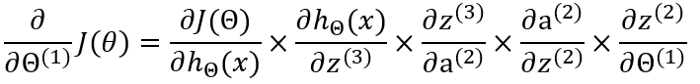
def back_propagation(self, h):
diff_J_wrt_h = -(np.divide(self.Y, h) - np.divide((1 - self.Y), (1 - h)))
diff_h_wrt_Z2 = h * (1 - h)
diff_J_wrt_Z2 = diff_J_wrt_h * diff_h_wrt_Z2
diff_J_wrt_A1 = diff_J_wrt_Z2.dot(self.params['theta_2'].T)
diff_J_wrt_theta_2 = self.params['A1'].T.dot(diff_J_wrt_Z2)
diff_J_wrt_b2 = np.sum(diff_J_wrt_Z2, axis = 0)
diff_J_wrt_Z1 = diff_J_wrt_A1 * (self.params['A1'] * ((1-self.params['A1'])))
diff_J_wrt_theta_1 = self.X.T.dot(diff_J_wrt_Z1)
diff_J_wrt_b1 = np.sum(diff_J_wrt_Z1, axis = 0)
self.params['theta_1'] = self.params['theta_1'] - self.learning_rate * diff_J_wrt_theta_1
self.params['theta_2'] = self.params['theta_2'] - self.learning_rate * diff_J_wrt_theta_2
self.params['b1'] = self.params['b1'] - self.learning_rate * diff_J_wrt_b1
self.params['b2'] = self.params['b2'] - self.learning_rate * diff_J_wrt_b2
def fit(self, X, Y):
self.X = X
self.Y = Y
self.init_weights()
for i in range(self.iterations):
h, cost = self.forward_prop()
self.back_propagation(h)
self.cost.append(cost)
def predict(self, X):
Z1 = X.dot(self.params['theta_1']) + self.params['b1']
A1 = self.sigmoid(Z1)
Z2 = A1.dot(self.params['theta_2']) + self.params['b2']
pred = self.sigmoid(Z2)
return np.round(pred)
def acc(self, y, h):
acc = (sum(y == h) / len(y) * 100)
return acc
def plot_cost(self):
fig = plt.figure(figsize = (10,10))
plt.plot(self.cost)
plt.xlabel('No. of iterations')
plt.ylabel('Logistic Cost')
plt.show()
The result of the above code would be a model with 3 layers. The input layer contained 30 inputs with 30 neurons or units each. The hidden layer contained a default 14 neutrons and the output layer contained the predicted 2 units for 0 and 1.
The training and learning step began after the learning rate was set to 0.001 and the number of epoch to 100.
The weights were randomly initialized with the bias weight standing apart and untouched. Next, both the sigmoid activation function and cost function were defined.
The forward propagation function was then determined by passing parameters from one layer to the next until they got to the output layer. Finally, the backpropagation was defined and the gradient descent was calculated. The result was used to update the weights.
The plot obtained for the cost function is shown below:
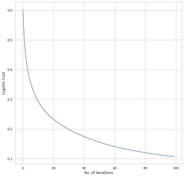
We can see how the cost functions continue to decrease with more epochs. We checked to see the level of accuracy of both the testing and training datasets.
Train accuracy: [97.14285714]
Test accuracy: [97.36842105]
The high amount of information or features available is responsible for such high accuracy.
What Methods Are Used to Build a Neural Network
Aside from understanding the neural network basics, it is also important to understand the methods for building both non-linear and linear neural network models.
The most vital part of building a model is matrix multiplication. We will consider 5 methods for carrying out this multiplication.
Simple Programme with Python
This is one method for carry out matrix multiplication. However, it is a very slow method. It can be performed using the code below:
In [0]:
 def matmul(a,b):
    ar,ac = a.shape # n_rows * n_cols
    br,bc = b.shape
    assert ac==br
    c = torch.zeros(ar, bc)
    for i in range(ar):
        for j in range(bc):
            for k in range(ac): # or br
                c[i,j] += a[i,k] * b[k,j]
    return c
PyTorch Element-wise Operations
This method of NN modeling can be used to build a pytorch neural network easily and quickly:
In [0]: def matmul(a,b):
    	    ar,ac = a.shape
   	    br,bc = b.shape
    	    assert ac==br
    	    c = torch.zeros(ar, bc)
    	    for i in range(ar):
        	for j in range(bc):
            	    # Any trailing ",:" can be removed
           	    c[i,j] = (a[i,:] * b[:,j]).sum() # running in C
    return c
NumPy Array Broadcasting
Here, we can use the C language instead of Python for vectorising and looping array operations:
m1[2].unsqueeze(1).shape
= torch.Size([784, 1])
Einstein Summation
By using this function, einsum, in a NumPy package we can easily sums and products in a generalized method.
%timeit -n 10 _=matmul(m1, m2)
PyTorch Operations
This method can use direct operators or functions to perform multiplication of matrices.
%timeit -n 10 t2 = m1. matmul(m2)Tutorial of NN Modeling
The following is a simplified tutorial for building a neural network for dummies. We will start from scratch. We shall begin by using the matrix multiplication process which we will refer to as MatMul. MatMul is a straightforward way to create the linear layers of the model.
We will employ the MNIST dataset from Fastai for the purpose of this tutorial. Using the lines of code below we will get the dataset:
In [0]:from pathlib import Path
   from IPython.core.debugger import set_trace
	from fastai import datasets
	import pickle, gzip, math, torch, matplotlib as mpl
	import matplotlib.pyplot as plt
	from torch import tensor

	MNIST_URL='http://deeplearning.net/data/mnist/mnist.pkl'

In [0]: path = datasets.download_data(MNIST_URL, ext='.gz');

In [0]:with gzip.open(path, 'rb') as f:
((x_train, y_train), (x_valid, y_valid), _) = pickle.load(f, encoding    ='latin-1')

In [0]:x_train,y_train,x_valid,y_valid = map(tensor,    (x_train,y_train,x_valid,y_valid))
The above code will download the dataset in NumPy array from which we can then access using the pickle.load function. We will need to employ PyTorch tensors to perform certain tasks, hence we will need to map the NumPy array to torch tensors using the map function.
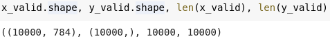
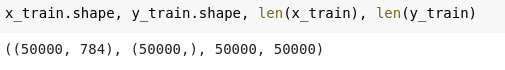
Once that step is complete, we can then divide 80% of our dataset into testing data and training data using the codes below.
Testing code:
Training code:
Next, we randomly initialize the weights and assign them accordingly:
weights = torch.randn(784,10)
bias = torch.zeros(10)

m1 = x_valid[:5]
m2 = weights

m1.shape,m2.shape
  = (torch.Size([5, 784]), torch.Size([784, 10]))
We then define the sigmoid activation function and the cost function using the 2 snippets of codes below.
def relu_grad(inp, out):
# grad of relu with respect to input activations
inp.g = (inp>0).float() * out.g
def mse_grad(inp, targ):
# grad of loss with respect to output of previous layer
inp.g = 2. * (inp.squeeze() - targ).unsqueeze(-1) / inp.shape[0]
The next step is to define both the forward and back propagation.
def forward_and_backward(inp, targ):

# forward pass:
    l1 = inp @ w1 + b1
    l2 = relu(l1)
    out = l2 @ w2 + b2
    # we don't actually need the loss in backwards!
    loss = mse(out, targ)

# backward pass:
    mse_grad(out, targ)
    lin_grad(l2, out, w2, b2)
    relu_grad(l1, l2)
    lin_grad(inp, l1, w1, b1)
forward_and_backward(x_train, y_train)Once the above steps are successful, we can now begin training our model to attain even higher accuracy by using the code below:
from torch import nn
class Model(nn.Module):
def __init__(self, n_in, nh, n_out):
super().__init__()
self.layers = [nn.Linear(n_in,nh), nn.ReLU(),
nn.Linear(nh,n_out)]
def __call__(self, x):
for l in self.layers: x = l(x)
return x
Conclusion
Building a NN model from scratch is indeed a huge task and there is a lot you need to know to succeed at it.
We recommend that you subscribe to our email newsletter so as to not miss any updates that will arise on this subject. Also, share this article with all your friends if you think it will bring them real value.