Stochastic Gradient Descent Vs Gradient Descent: A Head-To-Head Comparison

As the benefits of machine learning are become more glaring to all, more and more people are jumping on board this fast-moving train. And one way to do machine learning is to use a Linear Regression model. A Linear Regression model allows the machine to learn parameters such as bias terms and weight to find the global minimum or optimal solution while keeping the learning rate very low. By definition, the type of algorithms used in the Linear Regression model has the tendency to minimize error functions by iteratively moving towards the direction of the steepest descent as it is defined by the negative of whichever gradient we are using. Although Linear Regression can be approached in three (3) different ways, we will be comparing two (2) of them: stochastic gradient descent vs gradient descent. This will help us understand the difference between gradient descent and stochastic gradient descent.

What Are the Types of Gradient Descents?

There are primarily three (3) types of gradient descent. And they include:

1. Gradient Descent: The gradient descent is also known as the batch gradient descent. This optimization algorithm has been in use in both machine learning and data science for a very long time. It involves using the entire dataset or training set to compute the gradient to find the optimal solution. Our movement towards the optimal solution, which could be the local or global optimal solution, is always direct. Using this variant of the model to update for a parameter in a particular iteration requires that we run through all the samples of our training set every time we want to create a single update.

However, this can become a major challenge when we have to run through millions of samples. And because a gradient descent example involves running through the entire data set during each iteration, we will spend a lot of time and computational strength when we have millions of samples to deal with. Not only is this difficult, but it is also very unproductive.

2. Stochastic Gradient Descent: What is stochastic gradient descent (or SGD, for short)? SGD is a variant of the optimization algorithm that saves us both time and computing space while still looking for the best optimal solution. In SGD, the dataset is properly shuffled to avoid pre-existing orders then partitioned into m examples. This way the stochastic gradient descent python algorithm can then randomly pick each example of the dataset per iteration (as opposed to going through the entire dataset at once). A stochastic gradient descent example will only use one example of the training set for each iteration. And by doing so, this random approximation of the data set removes the computational burden associated with gradient descent while achieving iteration faster and at a lower convergence rate. The process simply takes one random stochastic gradient descent example, iterates, then improves before moving to the next random example. However, because it takes and iterates one example at a time, it tends to result in more noise than we would normally like.

3. Mini-Batch Gradient Descent: A mini-batch gradient descent is what we call the bridge between the batch gradient descent and the stochastic gradient descent. The whole point is like keeping gradient descent to stochastic gradient descent side by side, taking the best parts of both worlds, and turning it into an awesome algorithm. So, while in batch gradient descent we have to run through the entire training set in each iteration and then take one example at a time in stochastic, mini-batch gradient descent simply splits the dataset into tiny batches. Hence, it is not running through the entire sample at once, neither is it taking one example at a time. This creates some sort of balance in the algorithm where we can find both the robustness of stochastic and the computational efficiency of batch gradient descent.

Formulas of Gradient Descents

The first step in using the gradient descent algorithm is to assign small values to parameters. And as the algorithm begins to iterate moving towards finding the global minimum these values will keep changing. We are going to assume that the most important parameters are w (weight) and b (bias).

Once we have assigned values to the above parameters, we will have to pick a value for α (learning rate). We must be careful to pick a value that is neither too small nor too large. This is because if the number is large, then we will see the iteration diverge and overshoot, and if it too small we will notice an iteration that is slow and takes too long to converge towards the global minimum. To help us pick the right learning rate, therefore, there is the need to plot a graph of cost function against different values of α. Such a plot will look like the one below:

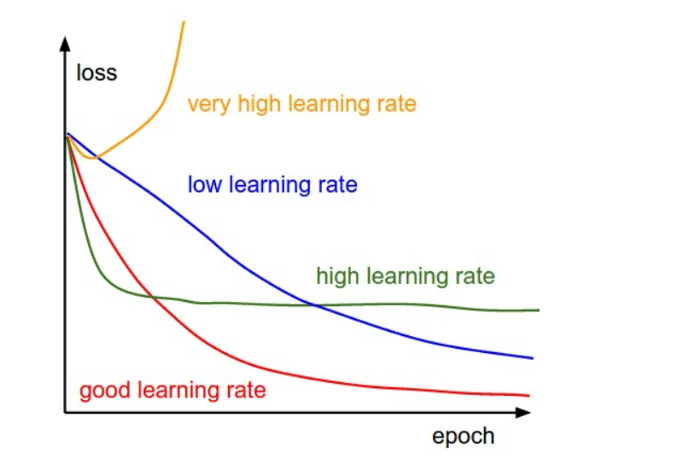
It is recommended to start by picking a value as small as 0.001 and going up from there. For instance, we can use the values 0.001, 0.003, 0.01, 0.03, 0.1, 0.3 and so on.

The formula for Batch Gradient Descent

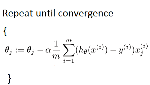
Like we had earlier discussed, the batch gradient descent takes the sum of all the training set to run a single iteration. The formula will then be:

The relationship below best describes how to initialize parameters in a batch gradient descent:

Below is a piece of batch gradient descent python code:

import numpy as np
import random


def gradient_descent(alpha, x, y, ep=0.0001, max_iter=10000):
    converged = False
    iter = 0
    m = x.shape[0] # number of samples


    # initial theta
    t0 = np.random.random(x.shape[1])
    t1 = np.random.random(x.shape[1])


    # total error, J(theta)
    J = sum([(t0 + t1*x[i] - y[i])**2 for i in range(m)])


    # Iterate Loop
    while not converged:
        # for each training sample, compute the gradient (d/d_theta j(theta))
        grad0 = 1.0/m * sum([(t0 + t1*x[i] - y[i]) for i in range(m)]) 
        grad1 = 1.0/m * sum([(t0 + t1*x[i] - y[i])*x[i] for i in range(m)])


        # update the theta_temp
        temp0 = t0 - alpha * grad0
        temp1 = t1 - alpha * grad1
    
        # update theta
        t0 = temp0
        t1 = temp1


        # mean squared error
        e = sum( [ (t0 + t1*x[i] - y[i])**2 for i in range(m)] ) 


        if abs(J-e) <= ep:
            print 'Converged, iterations: ', iter, '!!!'
            converged = True
    
        J = e   # update error 
        iter += 1  # update iter
    
        if iter == max_iter:
            print 'Max interactions exceeded!'
            converged = True


    return t0,t1

The formula for Stochastic Gradient Descent

With this variant of the algorithm, we usually run one example of the training set per iteration. Learning occurs after each iteration so that the parameters are updated after each operation (x^i,y^i). A stochastic gradient descent has the formula given below:

We may then see a stochastic gradient descent explained through the relationship below:

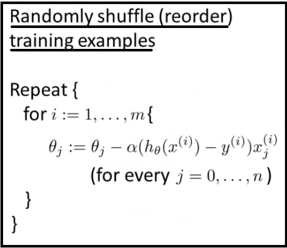
m here represents the number of training examples.

The formula for Mini-Batch Gradient Descent

The mini-batch gradient descent takes the operation in mini-batches, computingthat of between 50 and 256 examples of the training set in a single iteration. This yields faster results that are more accurate and precise. The mini-batch formula is given below:

When we want to represent this variant with a relationship, we can use the one below:

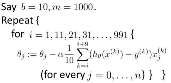
b here represents the number of batches while m represents the number of training examples.

Comparison of Stochastic Gradient Descent and Gradient Descent

A direct comparison of stochastic gradient descent vs gradient descent is important. Knowing the pros and cons of coordinate descent vs gradient descent will help highlight the advantages and disadvantages of both variants after which we can decide which one of them is more preferable.

Stochastic Gradient Descent

Pros:

• Computes faster since it goes through one example at a time
• The randomization helps to avoid cycles and repeat of examples
• Lesser computation burden which allows for lower standard the error
• Because the example size is less than the training set, there tends to be more noise which allows for the improved generalization error

Cons:

• It is usually noisier and this can result in a longer run time
• Results in larger variance because it works with one example per iteration

Gradient Descent (Batch Gradient Descent)

Pros:

• The trajectory towards the global minimum is always straightforward and it is always guaranteed to converge
• Even while the learning process is ongoing, the learning rate can be fixed to allow improvements
• It produces no noise and gives a lower standard error
• It produces an unbiased estimate of the gradients

Cons:

• It is slower and takes too much time
• It is computationally expensive with a very high computing burden

How Gradient Descent is Used in Machine Learning and Data Science

Now that we have compared gradient descent vs stochastic, let us consider the numerous ways gradient descent can be applied in both machine learning and data science because we already know that python stochastic gradient descent has been in application in several fields including machine learning for a very long time now.

Here are a few common ways we can apply gradient descent in both machine learning and data science:

• Support Vector Machine: Developed by Vapnik I, it uses a supervised learning algorithm for many forms of regression analysis.
• Logistic Regression applies logic not only to machine learning but to other fields including the medical field.
• Probabilistic Graphical Model: Which uses graphical representations to explain the conditional dependence that exists between various random variables.

Conclusion

To compare stochastic gradient descent vs gradient descent will help us as well as other developers realize which one of the dual is better and more preferable to work with. For many, the most significant difference between coordinate descent vs gradient descent is how less expensive it is to use stochastic gradient descent. This reason and many others is probably why stochastic gradient descent, especially, continues to gain increasing acceptance in machine learning and data science.

Remember that you can subscribe to our email newsletter and follow the discussion even as we continue to expound on similar concepts. Lastly, you can go ahead share this article with your friends on all social media so they too can gain value.